
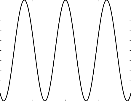
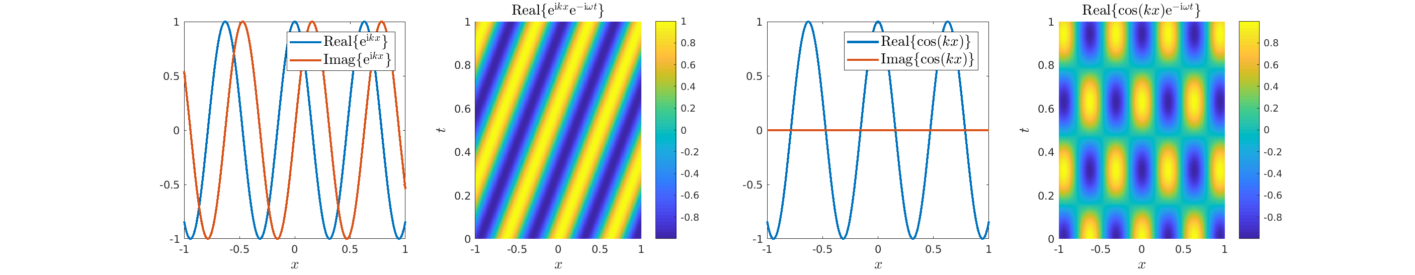
Solutions of the Helmholtz equation in 1 dimension: propagative wave \(u(x)=\mathrm e^{\mathrm ikx}\) and standing wave \(u(x)=\cos(kx)=\frac{\mathrm e^{\mathrm ikx}+\mathrm e^{-\mathrm ikx}}2\), and their evolution in time \(U(x,t)=\Re\{u(x) \mathrm e^{-\mathrm ikt}\}\).
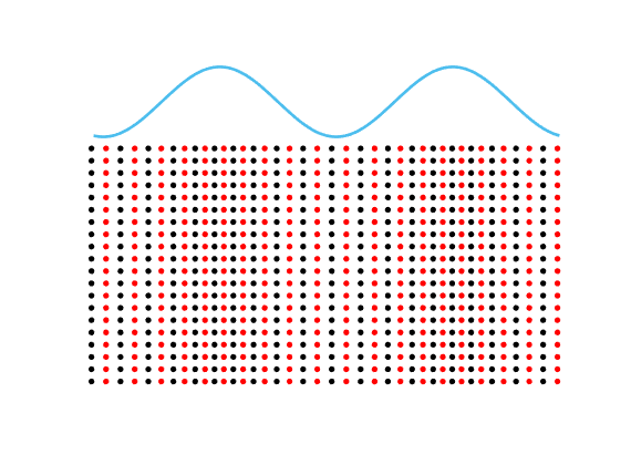
Motion of the particles in a fluid subject to an acoustic plane wave \(U(\mathbf{x},t)=\cos(k(x_1-ct))\).
Each particle oscillates harmonically back and forth, but remains in a small region.
The blue line represents the acoustic pressure (or the density).
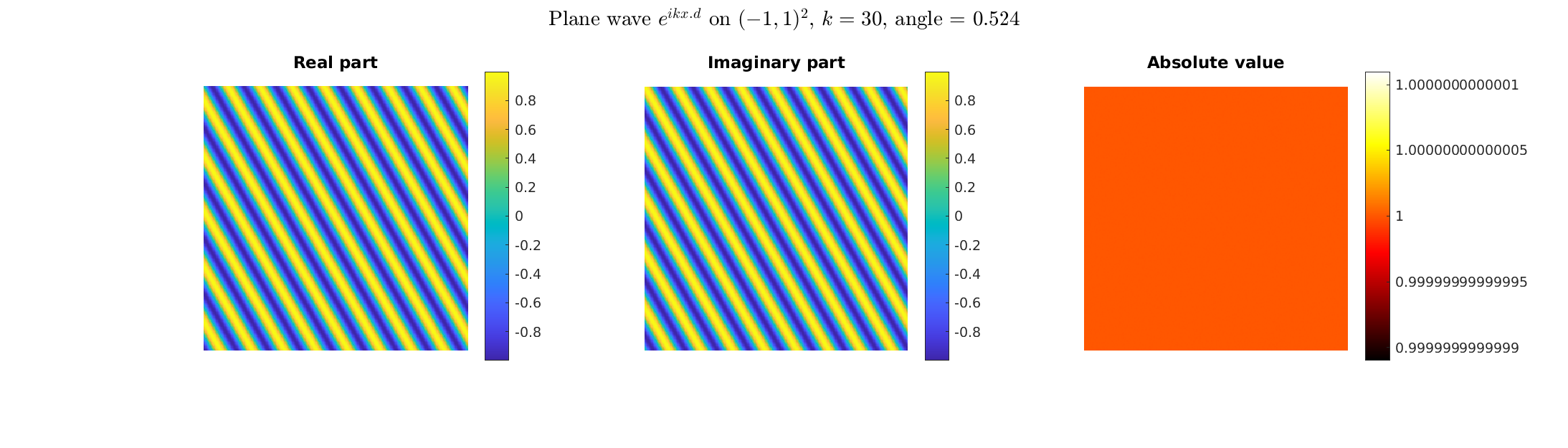
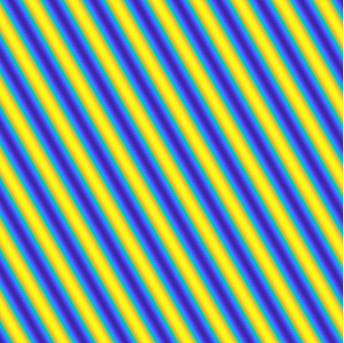
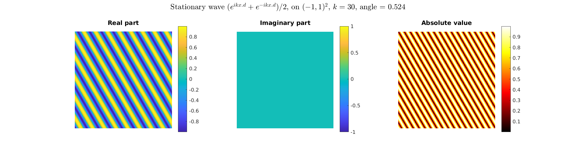
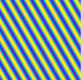
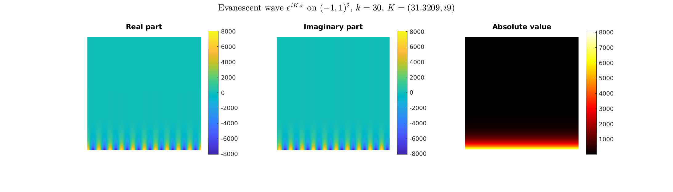
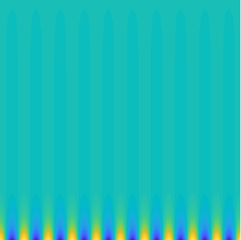
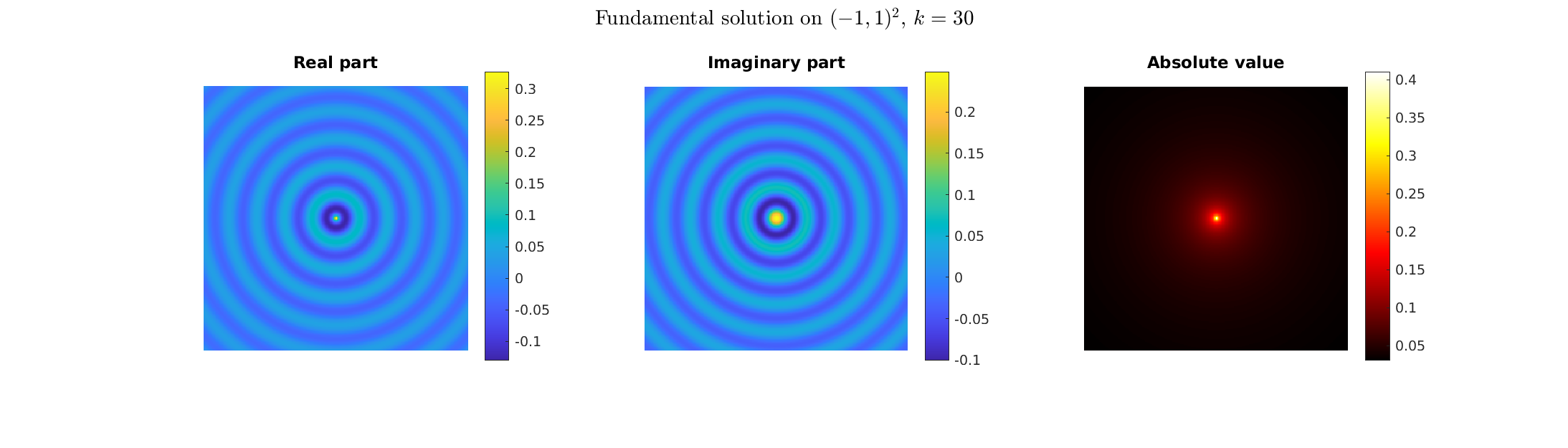
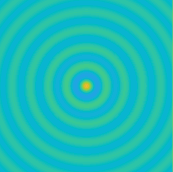
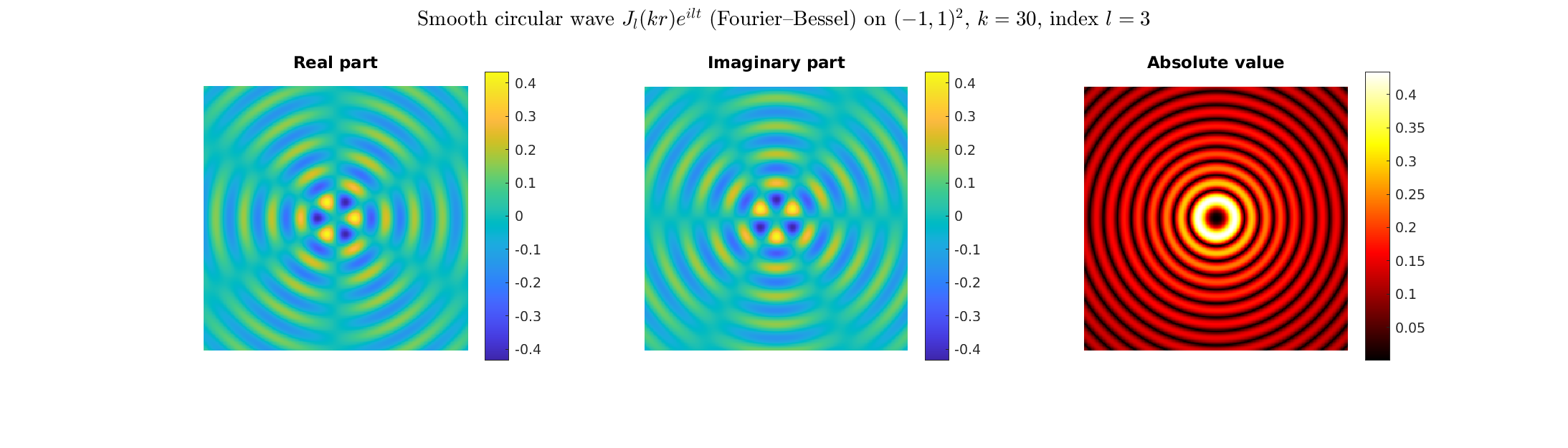
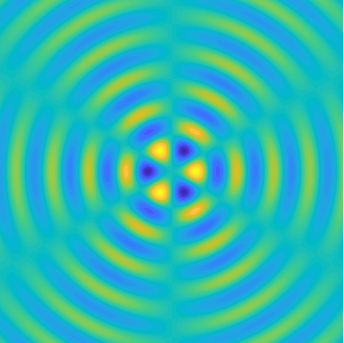
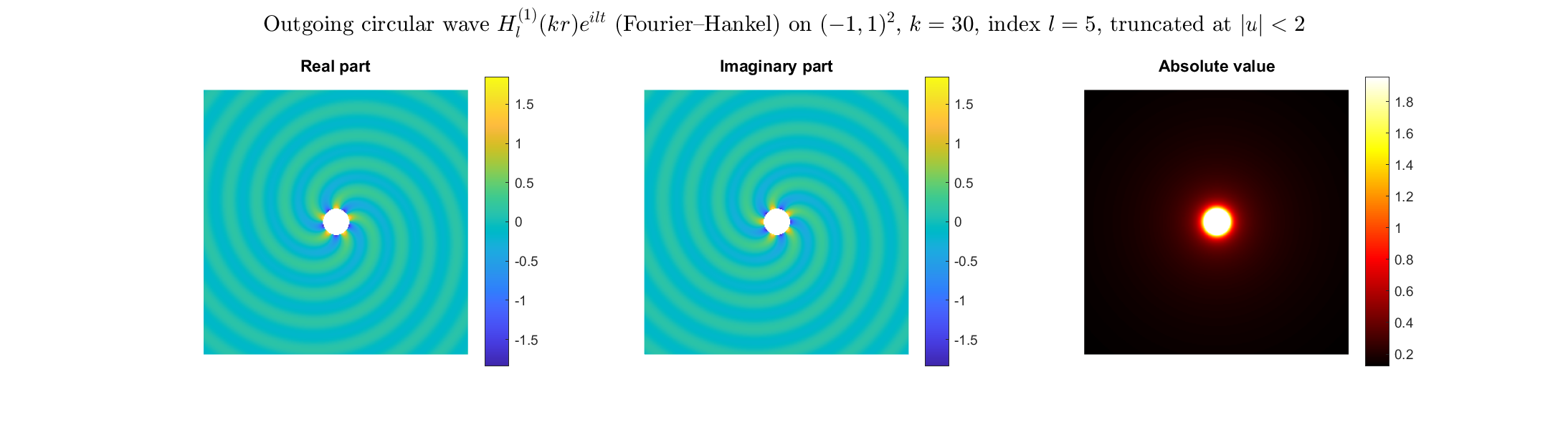
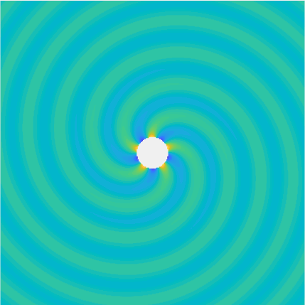
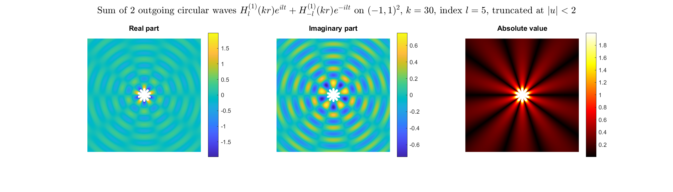
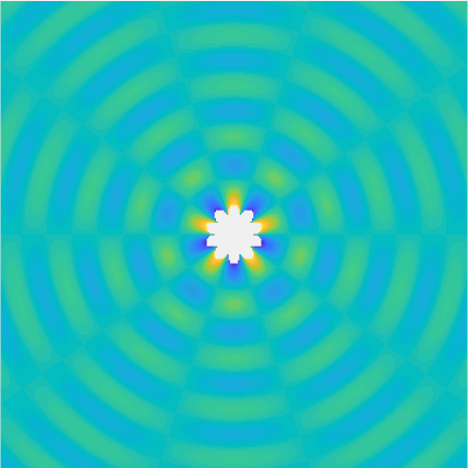
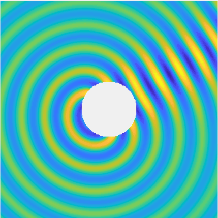
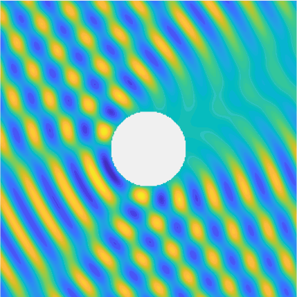
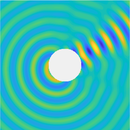
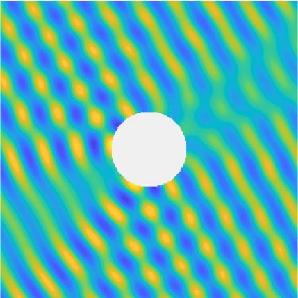
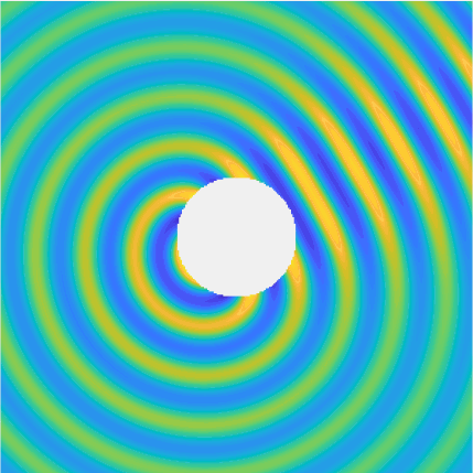
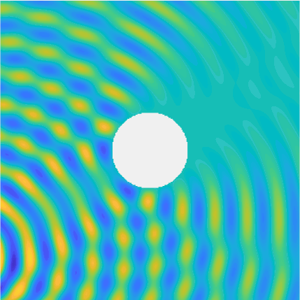
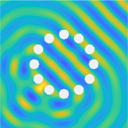
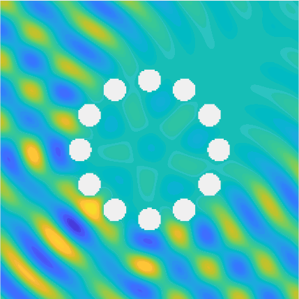
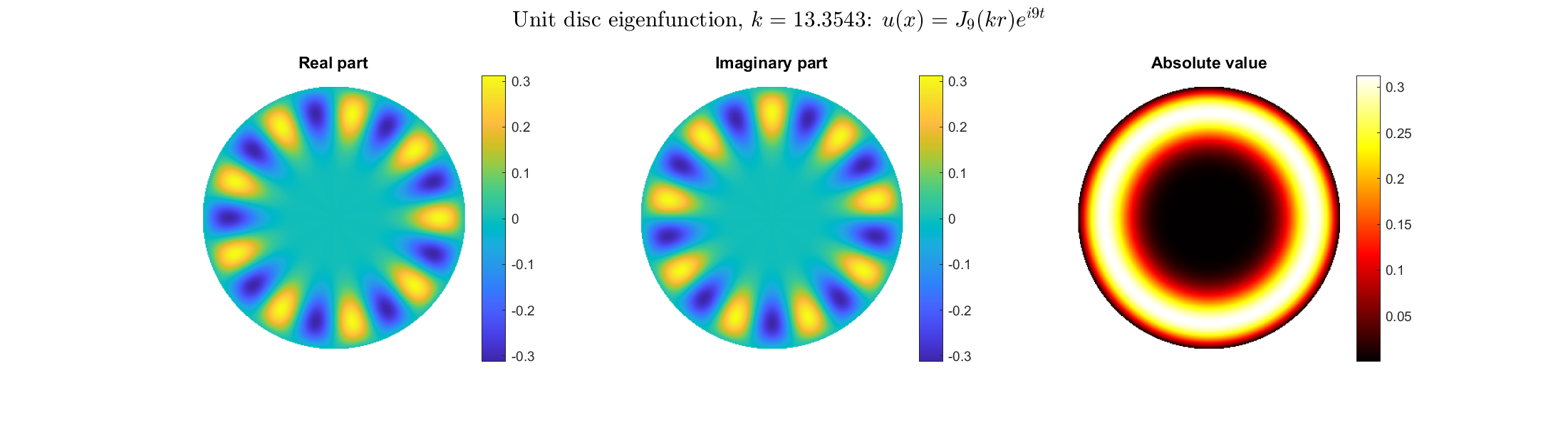
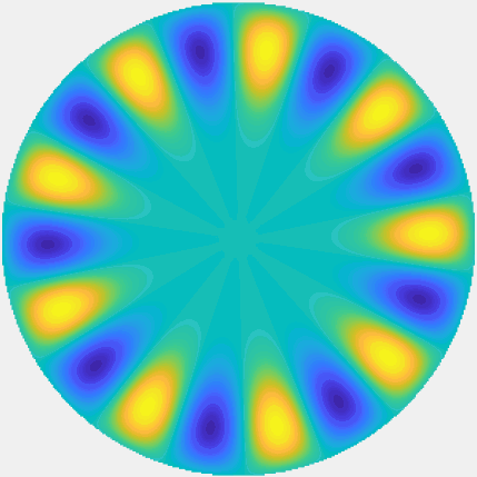
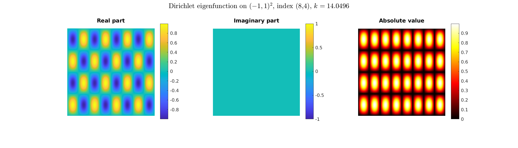
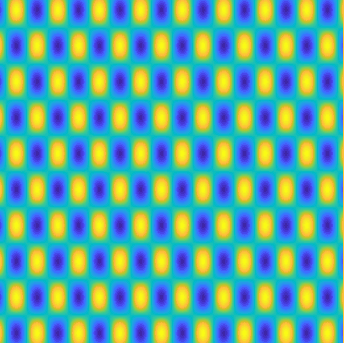
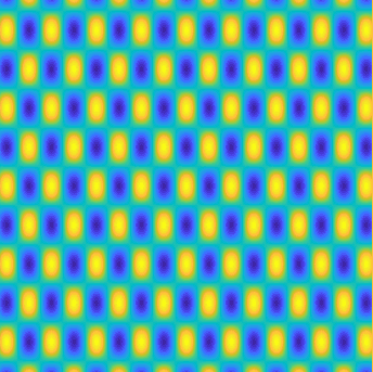
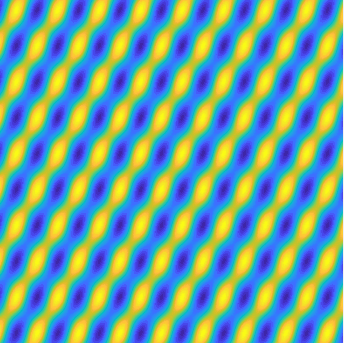
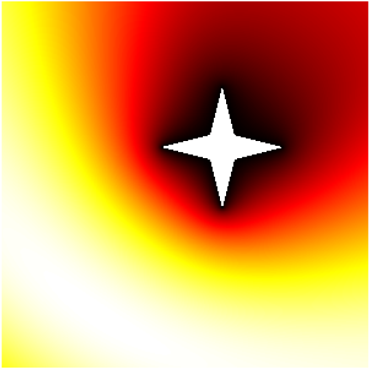
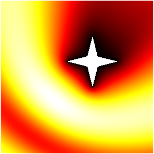
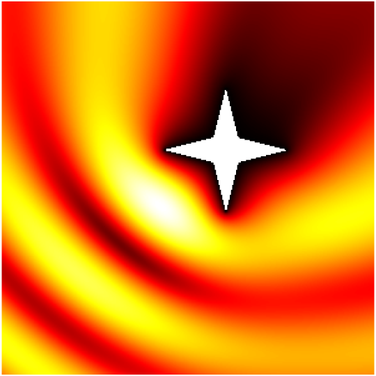
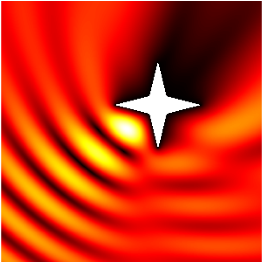
Special solutions of the Helmholtz equation in 2 dimensions: real and imaginary parts, magnitude and time evolution.
|
|
|
|
|
|
|
|
|
|
|
|
|
|
|

|
|
|
|
Solutions of the Helmholtz equation in 2 dimensions: plane wave of direction \((\frac{\sqrt3}2,-\frac12)\) reflected by horizontal line.
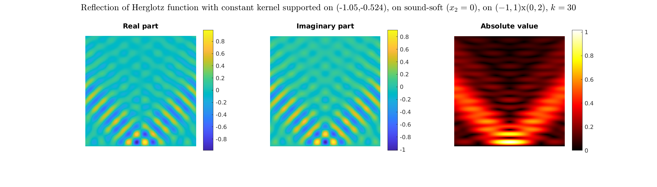
On the lower side of the square we have imposed sound-soft (\(u=0\)), sound-hard (\(\partial_n u=0\))
and impedance (\(\partial_n u-\mathrm ik\vartheta u=0\), \(\vartheta=1\)) boundary conditions, respectively.
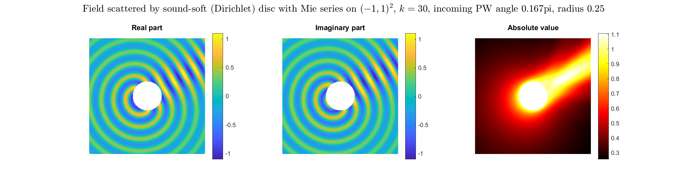
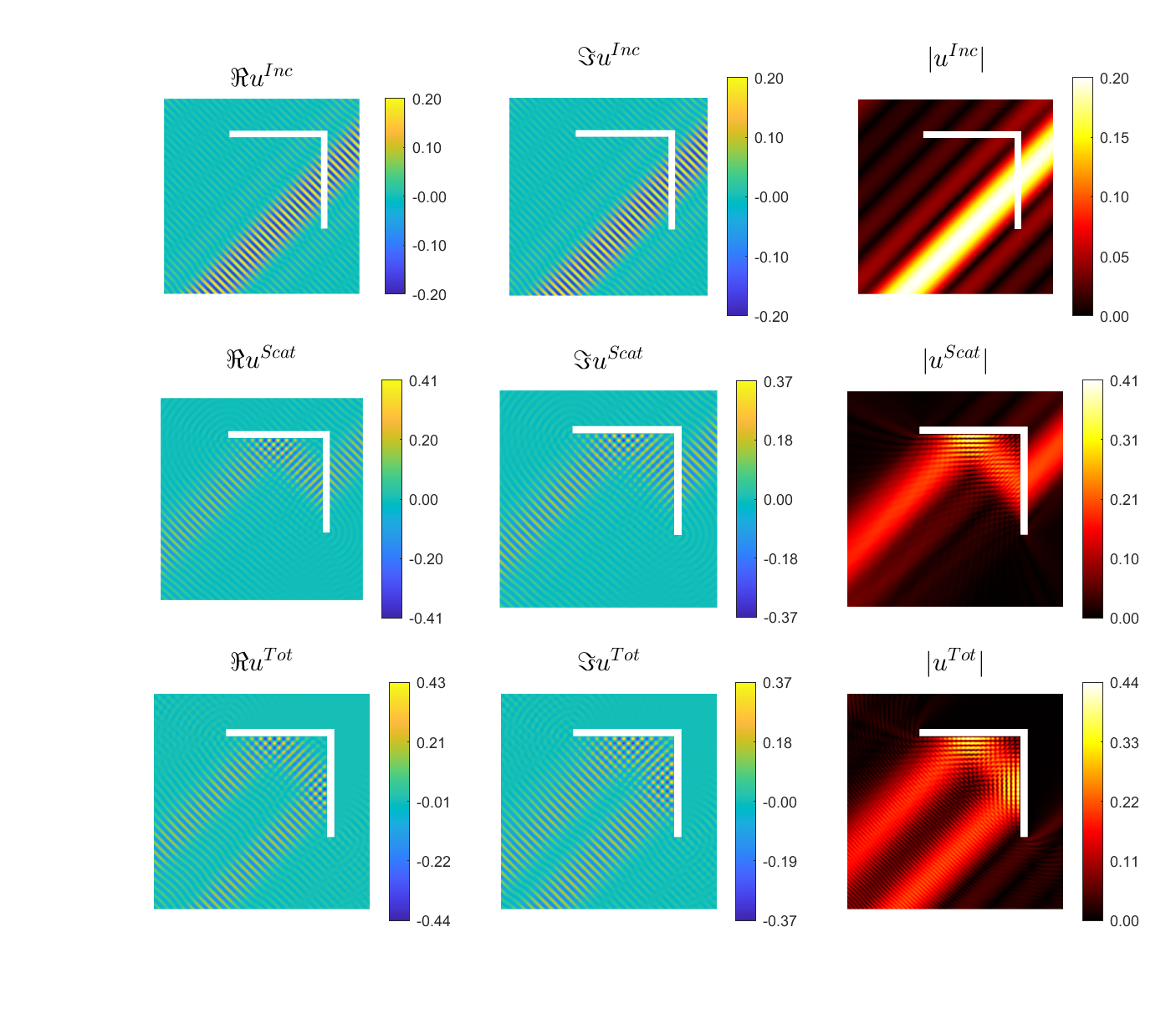
Examples of BEM computations: scattering of a plane wave of direction \((\frac12,\frac{\sqrt3}2)\) by sound-soft polygons.
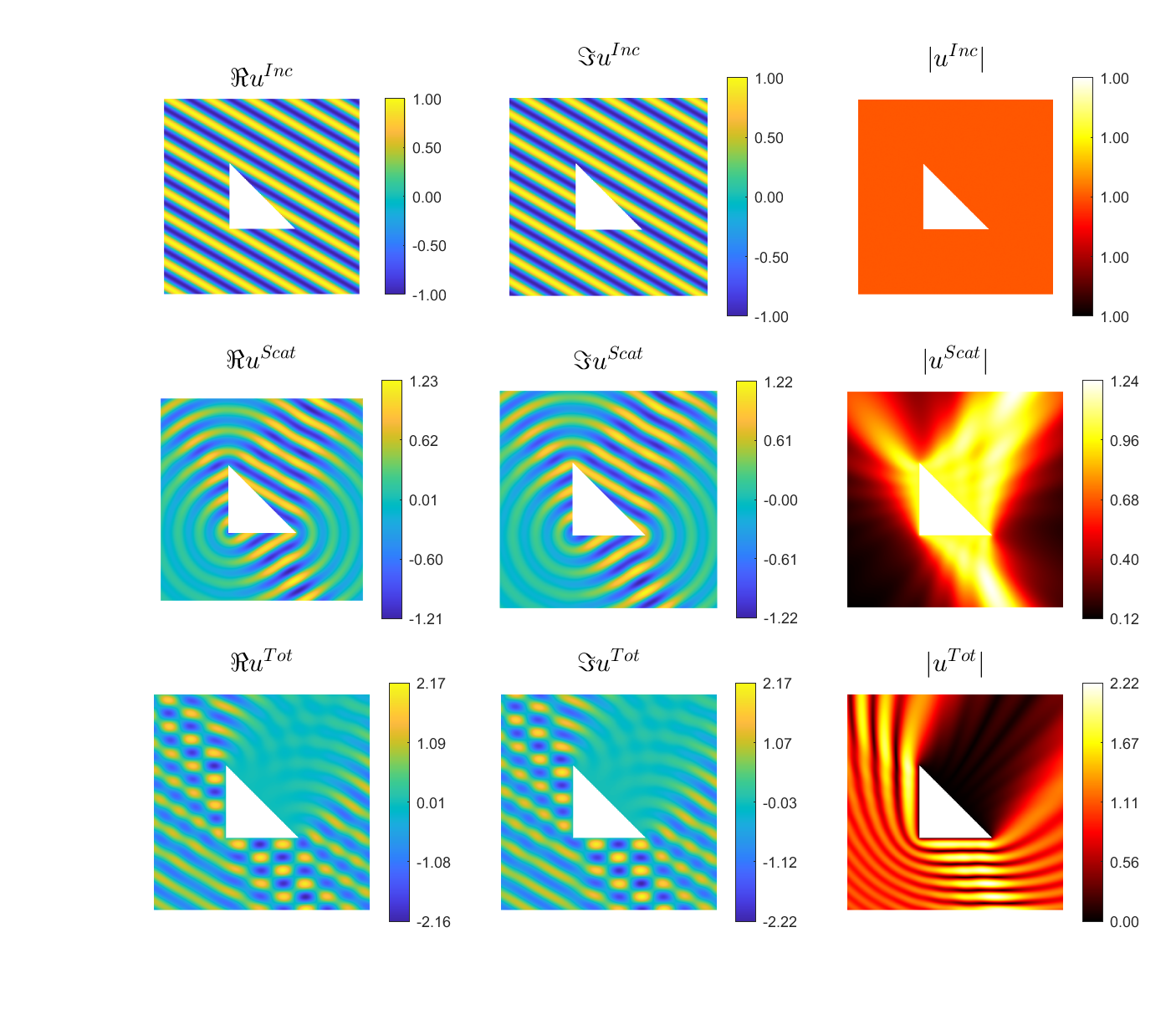 |
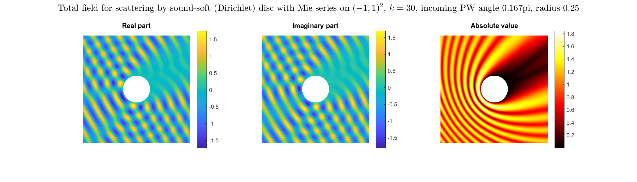
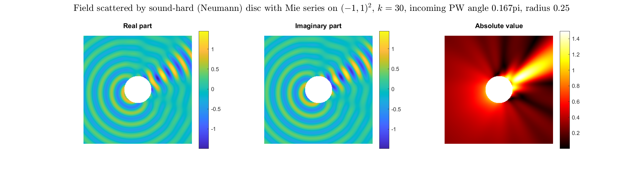
Scattered field: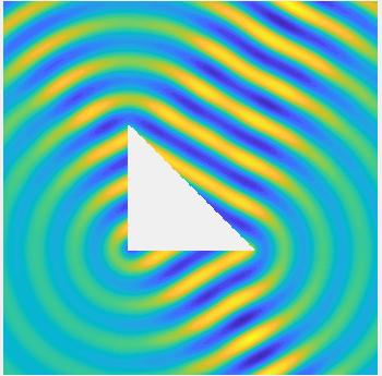
Total field: 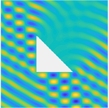
|
 |
Scattered field: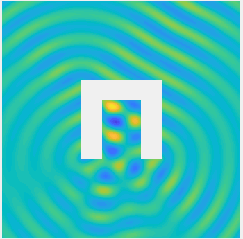
Total field: 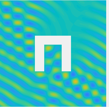
|
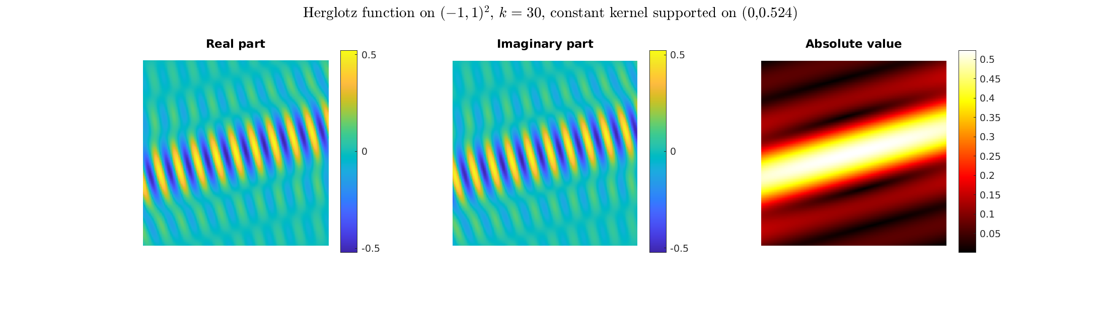
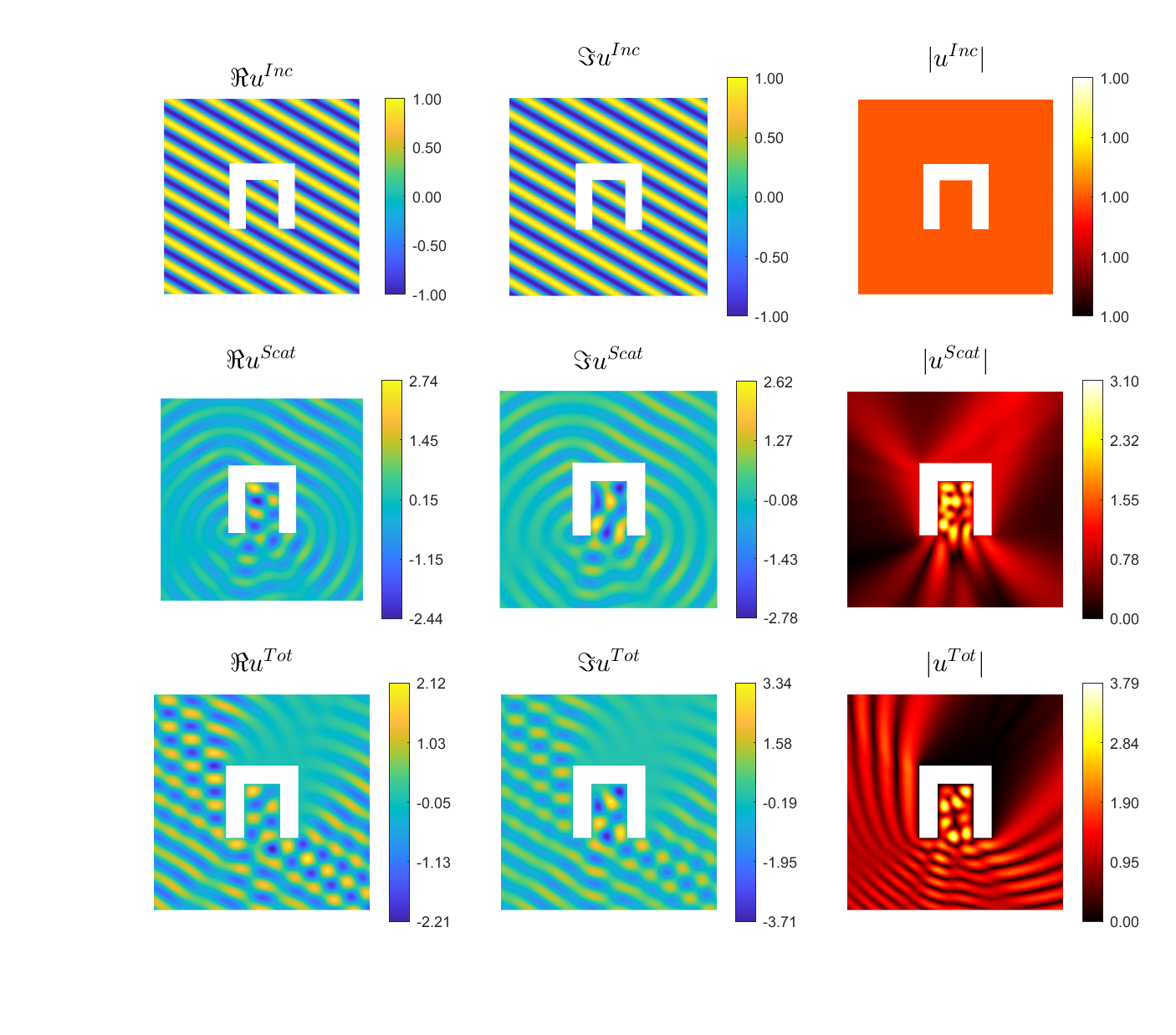
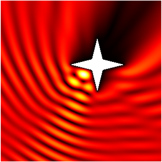
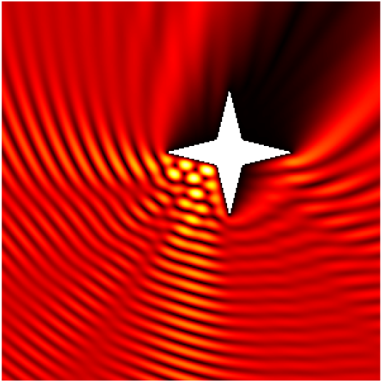
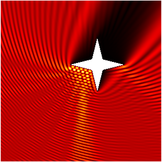
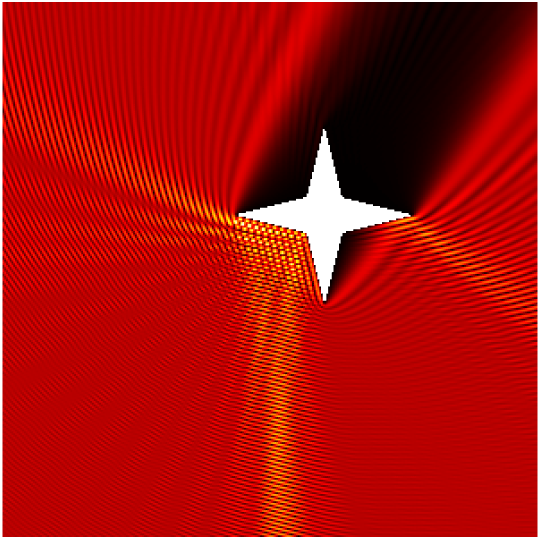
Scattering of a Herglotz function \(u^{Inc}(\mathbf{x})= \int_{\frac\pi4-\frac1{10}}^{\frac\pi4+\frac1{10}}e^{ik((x_1-0.7)\cos\varphi+x_2\sin\varphi)}d\varphi\) by \((0,1.5)^2\setminus(0,1.4]^2\), with \(k=70\), plotted on \((-1,2)^2\).
 |
Scattered field: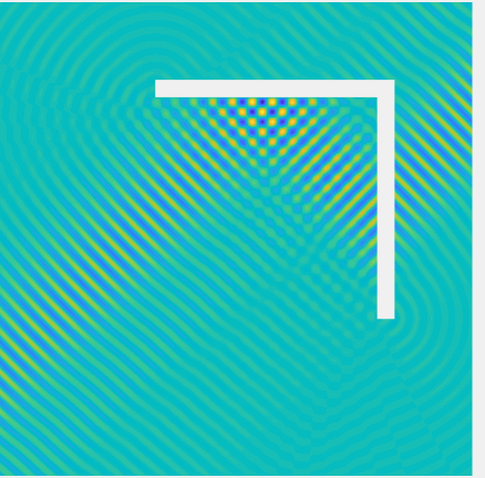
Total field: 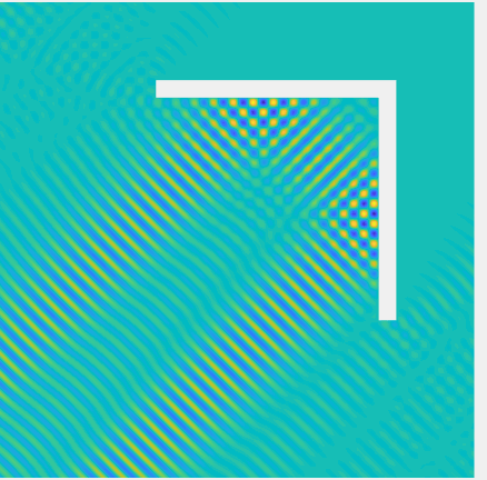
|
Scattering by the same non-convex obstacle of plane waves with direction \((\frac12,\frac{\sqrt3}2)\) and wavenumbers \(k=1,2,4,8,16,32,64,128\) (total field magnitude).
Back to the "Advanced numerical methods for PDEs" page.
The Matlab file used to generate most of the figures and the animations (excluding those computed with the BEM):
MNAPDEdrawwaves.m
Benchmark to test the results of the BEM code: file .mat (computed with MPSpack).
Plenty of animations of 2D solutions of the wave equation, interpreted as dimensional reduction of the Maxwell equations, can be found on Robin Hogan's page:
http://www.met.reading.ac.uk/clouds/maxwell/
Other animations of acoustic and elastic waves can be found on the page of Daniel A. Russell:
https://www.acs.psu.edu/drussell/demos.html
A simple interactive introduction to sound propagation is on the page of Bartosz Ciechanowski:
https://ciechanow.ski/sound/